Layer Geometry

Introduction

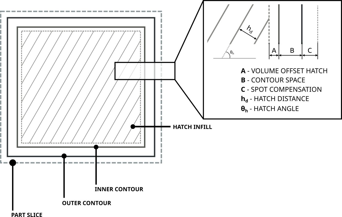
In PySLM, the foundation for generating the scan paths for L-PBF is based on a common format for representing the geometry of a layer within the ‘machine build files’ used across the majority of commercial LPBF systems. The typical infill pattern consists of a series of boundaries obtained by slicing that are offset and the interior region infilled with hatch vectors, constantly spaced with hatch distance \(h_d\) and orientated at hatch angle \(\theta_h\). The offsets of the boundary are arbitrarily chosen but often compensate for the beam size and additional offsetting to reduce the likelihood for producing porosity and other defects due to instability in the process.

Subtly, the scan paths are more concise definition and do not follow the typical G-CODE format used across other 3D printing systems. However, there is a tendency that the definition the scan paths will follow a similar pattern, that is mostly historically driven by the early L-PBF systems and those based on the original .cli specification.

The structure of machine build file is that composed from the following sections:

• Header,

• Models,

• Layers .

The header contains machine specific metadata, and parameters for controlling the build.The models section contains details about individual parts within a build and a selection of Laser Parameters grouped as Build Style. Finally, as this remains a planar process the layers section, at a prescribed build height in the \(Z\) direction. Each layer contains the various 2D layer geometry that describe the infill raster pattern used for controlling the scan-paths taken by the exposure sources. The common layer geometry types are 1D exposures or 2D scan vectors that are linearly discretised across the layer:

• Hatches

• Contours / Boundaries

• Points

Geometry Structure

PySLM builds upon these structures throughout to provide a universal interface for generating layer geometry features (i.e. scan-vectors) and subsequent translation to associated machine build files that can be utilised across a range of commercial L-PBF systems via libSLM and simulation tools. These structures are defied in the pyslm.geometry module, which will transparently load libSLM if available.

Parts and their Laser Parameters are contained within Model. Each model at a minimum must contain a unique mid (model id) and the topLayerId. The top layer id identifies the uppermost layer that contains the highest Z value for any LayerGeometry that is associated for a model group. The model can also contain a list of BuildStyle that define the choice of laser parameters.

Note

Currently it is assumed that laser parameters are assigned to a group of scan vectors. In future, some system support may be added to allow for the assignment of laser parameters to individual scan vectors.

A Model can be created as follows:

from pyslm.geometry import Model

# Create a model
model = Model(mid=1, topLayerId=10)

# Attribute can be seperately assigned
model.mid = 1
model.topLayerId = 10

Build Styles

Each build style contains a unique bid and a set of laser parameters typical across most L-PBF systems. These can be attached to each Model. The laser parameters are referenced by each LayerGeometry using their mid and bid references respectively. Therefore, it is required that each model contains at least one build style and are uniquely identifiable.

from pyslm.geometry import BuildStyle

bstyle = pyslm.geometry.BuildStyle()
bstyle.bid = 1
bstyle.laserSpeed = 200  # [mm/s]
bstyle.laserPower = 200  # [W]
bstyle.jumpSpeed  = 5000 # [mm/s]

# Create a second build style with a unique name
bstyle2 = pyslm.geometry.BuildStyle(bid=2)
bstyle2.laserSpeed = 200  # [mm/s]
bstyle2.laserPower = 200  # [W]

# Attached the build styles to the model
model.buildStyles.append([bstyle, bstyle2])

An additional set of laser parameters can be defined for each build style, which are specifically associated with the pyslm.analysis module, for calculating the build times and estimate energy consumption. These may not necessarily used by the L-PBF system when exported to the machine build files. These are defined as follows:

# Optional laser param
bstyle.jumpSpeed  = 5000 # [mm/s] - The jump speed used when jumping betwee scan vectors
bstyle.jumpDelay  = 10   # [mu s] - The jump delay used when jumping between scan vectors
bstyle.pointDelay = 10   # [mu s] - The point delay used when exposing a point (Pulsed laser systems)

The laser parameters are stored in the BuildStyle object and other machine specific parameters can be defined and are stated below for reference:

• pointExposureTime - Point Exposure Time [:math:`mu`s] for Pulsed Laser Systems

• pointDistance - Point Exposure Distance [:math:`mu`m] for Pulsed Laser Systems

• laserFocus - Laser focus position [mm] for some laser systems

• laserId - Laser ID for multi-laser systems

• description - A description of the build style

The parameters may be used during translation using libSLM.

Note

The laser parameters required to be specified is not exhaustive, and will depend on the L-PBF platform utilised. For example, depending on the laser type (CW, or Pulsed) the laser speed parameter may be defined, or the point exposure time and distance.

Each Layer contains a unique (layerId) and (z) position stored as microns. Within each layer, this stores the layer geometry, which is an ordered list of LayerGeometry features. These are processed in the order they are stored in pyslm.geometry.Layer.geometry.

LayerGeometry is a base class, and in practice derived geometry types can be used:

• HatchGeometry - Scan vectors defined by pair-wise coordinates with jumps between

• ContourGeometry - Scan vectors that are connected to form a closed loop

• PointsGeometry - A sequence of point exposures

Each geometry type must reference a BuildStyle and Model object using the bid and mid attributes respectively. Crucially, the coordinates defining the exposure points and vectors are stored in the coords. The coordinates are stored as a numpy array with shape (n, 2) where n is the number of points and are stored typically using mm.

Note

Typically for visualisation, hatch vectors are representing using a numpy array with shape (n,2,2) where n is the number of hatch vectors to represent the pair of coordinates.

The following example demonstrates how to create a layer geometry with a contour and hatch geometry for a single layer.

import pyslm.visualise
from pyslm.geometry import Layer, ContourGeometry, HatchGeometry

layer = Layer(layerId=1, z=30)

contourGeom = ContourGeometry()
contourGeom.mid = 1
contourGeom.bid = 1  # Use the first build style for hatch vectors
contourGeom.coords = np.array([[0., 0], [1., 0], [1., 1.], [0., 1.], [0., 0.]])

hatchGeom = geom.HatchGeometry()
hatchGeom.mid = 1
hatchGeom.bid = 2 # Use the second build style for hatch vectors
hatchGeom.coords = np.array([[0.1, 0.1], [0.9, 0.1], # Hatch Vector 1
                             [0.1, 0.3], [0.9, 0.3], # Hatch Vector 2
                             [0.1, 0.5], [0.9, 0.5], # Hatch Vector 3
                             [0.1, 0.7], [0.9, 0.7], # Hatch Vector 4
                             [0.1, 0.9], [0.9, 0.9]  # Hatch Vector 5
                            ])

# Append the layer geometry to the layer
layer.geometry = [hatchGeom, contourGeom]

Validation

Generated geometry can be validated using an additional utility ModelValidator . This class which will check the structures for consistency and ensure that the geometry is correctly defined throughout. This is important for large build files consisting multiple models and build styles, and difficulty identify problems that can occur when exporting to machine build files.

ModelValidator is supplied with a list of Layer and Model , and internally will check for consistency. The following short example demonstrates how to validate the geometry used as input prior to generating a machine build file:

import pyslm.geometry

# Create a list of models and a list of layers
models = [model]
layers = [layer]

""" Validate the input model """
pyslm.geometry.ModelValidator.validateBuild(models, layers)

Exporting

Once the build file structures are defined, these can be used to export to a machine build file format via libSLM. Additionally, these files can be imported back into PySLM and re-used for further analysis or visualisation. There are a variety of formats currently available including:

• Renishaw (.mtt)

• DMG Mori - Realizer (.rea)

• EOS (.sli)

• SLM Solutions (.slm)

• CLI (.cli) - Common Layer Interface

For further guidance, including installation please refer to the libSLM documentation. Generally, the process is very trivial once the prior structures has been generated. Additional information may be required specific to the L-PBF system, and additionally a header structure for defining additional build parameters or metadata. The following example demonstrates how to export the geometry to a Renishaw machine build file (.mtt):

from libSLM import mtt

"""
A header is needed to include an internal filename. This is used as a descriptor internally for the Machine Build File.
The translator Writer in libSLM will specify the actual filename.
"""
header = slm.Header()
header.filename = "MachineBuildFile"

# Depending on the file format the version should be provided as a tuple
header.version = (1,2)

# The zUnit is the uniform layer thickness as an integer unit in microns. Normally should be set to 1000
header.zUnit = 1000 # μm

""" Create the initial MTT Writer Object and set the filename"""
mttWriter = mtt.Writer()
mttWriter.setFilePath("build.mtt")
mttWriter.write(header, models, layers)

For other machine build file formats, these are constructed similarly, but will have specific parameters or modifications required to be accepted by the system. Likewise machine build files can be imported back into PySLM for further analysis or visualisation.

from libSLM import mtt
import pylsm.visualisation

mttReader = mtt.Reader()
mttReader.setFilePath("build.mtt")
mttReader.parse()

layers = mttReader.layers
pyslm.visualisation.plot(layers[0])